The Math and ActionScript of Curves: Drawing Quadratic and Cubic Curves

We see lines used in a lot of scenarios. Curves are also used, although perhaps not as frequently - but that doesn't undermine their importance! In this tutorial we shall take a closer look at curves, particularly the quadratic and cubic curve, along with some of their commonly used mathematical features.

Final Result Preview

Let's take a look at the final result we will be working towards. Drag the red dots and see the gradients change in position.

And here's another demo, using cubic curves, without the gradients:

Step 1: Curves

Quadratic and cubic will be featured in each of these sections. So let's first look at the equation of curves. These equations are written in polynomial form, starting with the term of highest degree. The first one is quadratic equation (highest degree is 2); the second is cubic equation (highest degree is 3).
\[f(x) = Ax^2 + Bx + C\ ... (eq\ 1)\]
\[g(x) = Ax^3 + Bx^2 + Cx + D\ ... (eq\ 2)\]

Note that A, B, C and D are real numbers. So now that we are aquainted with it, let's try to visualise it. Graphing curves will be our next attempt.

Step 2: Graphing Curves

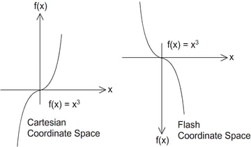
First, let's graph a quadratic curve. I'm sure all readers have graphed quadratic curve in high school math class, but just to refresh your memory, I present graphs below. They are placed side by side to ease comparison.

Left graph is using Cartesian coordinate space
Right graph is using Flash coordinate space

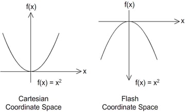
Graphing onto Cartesian and Flash coordinate spaces.

The obvious difference is the inverted y-axis on Flash coordinate space. They look simple overall, right? Okay, now we're ready to plot onto Flash coordinate space.

Step 3: Quadratic Coefficients

To position quadratic curves at the right spot, we need to understand their corresponding equations. The curve drawn is really dependant on the equation's coefficients (for the case of quadratic, those are A, B and C).

I've included a Flash presentation below so you can easily tweak these coefficients and get immediate feedback.

To study the effects of individual coefficients on the overall curve, I suggest following the steps below to experiment with the Flash presentation above.

While setting A and B to 0, tweak the value of C to both positive and negative values. You'll see the line's height change.
Now tweak the value of B between positive and negative values. Observe what happens to gradient of line.
Now tweak the value of A between positive and negative values, and compare the results.
Then tweak B between being positive and negative again. Observe the curve's always cutting through the origin.
Finally tweak C. Observe the whole curve shift along the y-axis.

Another interesting observation is that throughout the second and third steps of the above, the point of inflection (i.e. the turning point) stays at the same point on the y-axis.

Step 4: Alternative Equation One

You quickly see that positioning a curve is somewhat difficult. The equation used is impractical if we want to, say, locate the coordinates of the lowest point on a curve.

Solution? We'll rewrite the equation into a desired form. Check out the following equation:

\[f(x) = P(x+Q)^2+R\]

It's still a quadratic equation, but it's taken another form. Now we can easily control the minimum and maximum points on the curve. In the previous Flash presentation, click on button "Approach 1" on the top right and play with the new values.

Here's a brief explanation of the coefficients' roles:

Coefficient	Role
P	Control the curve's steepness.
Q	Control displacement of curve's turning point along x-axis.
R	Control displacement of curve's turning point along y-axis.

Nonetheless, it's still a difficult task to make the curve pass through a given set of points. We'd have to rigorously pre-calculate on paper before translating it to code.

Fortunately, there is a better solution. But before going through it, let's have a look at the ActionScript implementation as of now.

Step 5: ActionScript Implementation

Here are the equations written as ActionScript functions (check Graphing.as in the source download).


private function quadratic1(x:Number, A:Number, B:Number, C:Number):Number {
    //y = A(x^2) + B(x) + C
    return A*x*x+ B*x + C
}

private function quadratic2(x:Number, P:Number, Q:Number, R:Number):Number {
    // y = P * (x + Q)^2 + R
    return P*(x+Q)*(x+Q) + R
}

And here's an implementation of the drawing method using Graphics.drawPath(). Just a note that all curves in this article are drawn in similar fashion.

First the variables...

1
2	private var points:Vector.<Number> = new Vector.<Number>;
3	private var drawCommand:Vector.<int> = new Vector.<int>;

Now the y-positions, calculated based on the x-positions and the given coefficients.


private function redraw(A:Number, B:Number, C:Number):void {
    for (var i:int = 0; i < 400; i++) {
        var x:Number = i - 200;
        points[i * 2] = x * 10 + stage.stageWidth >> 1;
        if (isApproach1) {
            points[i * 2 + 1] = quadratic1(x, A, B, C) + stage.stageHeight >> 1
        }
        else {
            points[i * 2 + 1] = quadratic2(x, A, B, C) + stage.stageHeight >> 1
        }
        
        if (i == 0) drawCommand[i] = 1;
        else drawCommand[i] = 2;
    }
    graphics.clear();
    graphics.lineStyle(1);
    graphics.drawPath(drawCommand, points);
}

(Confused about the >> operator? Take a look at this tutorial.)

Step 6: Alternative Equation Two

Suppose we're given three points that the quadratic curve must cross through; how do we form the corresponding equation? More specifically, how can we determine the coefficient values of the equation? Linear algebra comes to the rescue. Let's analyse this problem.

We know that quadratic equations always take form as written in eq. 1 in Step 1.

\[f(x) = Ax^2 + Bx + C\ ... (eq\ 1)\]

Since all three coordinates given are lying on the same curve, they must each satisfy this equation, with the same coefficients as the equation of the curve that we are looking for. Let's write this down in equation form.

Given three coodinates:

\(S\ \left(S_x,\ S_y\right)\)
\(T\ \left(T_x,\ T_y\right)\)
\(U\ \left(U_x,\ U_y\right)\)

Substitute these values into (eq 1). Note that A, B, C are unknowns at the moment.

\[f(x) = Ax^2 + Bx + C\ ... (eq\ 1)\]

\(S_y = A\left(S_x\right)^2 + B\left(S_x\right) + C\ \)
\(T_y = A\left(T_x\right)^2 + B\left(T_x\right) + C\ \)
\(U_y = A\left(U_x\right)^2 + B\left(U_x\right) + C\ \)

Now, rewrite in matrix form. Take note that A, B, C are the unknowns we are solving for.

[latex]
\begin{bmatrix}S_y \\T_y \\U_y\end{bmatrix} =
\begin{bmatrix}
\left(S_x\right)^2 & \left(S_x\right) & 1\\
\left(T_x\right)^2 & \left(T_x\right) & 1\\
\left(U_x\right)^2 & \left(U_x\right) & 1\end{bmatrix}
\begin{bmatrix}A \\B \\C\end{bmatrix} \\
[/latex]

[latex]
\begin{bmatrix}
\left(S_x\right)^2 & \left(S_x\right) & 1\\
\left(T_x\right)^2 & \left(T_x\right) & 1\\
\left(U_x\right)^2 & \left(U_x\right) & 1\end{bmatrix}^{-1}
\begin{bmatrix}S_y \\T_y \\U_y\end{bmatrix} =
\begin{bmatrix}
\left(S_x\right)^2 & \left(S_x\right) & 1\\
\left(T_x\right)^2 & \left(T_x\right) & 1\\
\left(U_x\right)^2 & \left(U_x\right) & 1\end{bmatrix}^{-1}
\begin{bmatrix}
\left(S_x\right)^2 & \left(S_x\right) & 1\\
\left(T_x\right)^2 & \left(T_x\right) & 1\\
\left(U_x\right)^2 & \left(U_x\right) & 1\end{bmatrix}
\begin{bmatrix}A \\B \\C\end{bmatrix} \\
[/latex]
[latex]
\begin{bmatrix}
\left(S_x\right)^2 & \left(S_x\right) & 1\\
\left(T_x\right)^2 & \left(T_x\right) & 1\\
\left(U_x\right)^2 & \left(U_x\right) & 1\end{bmatrix}^{-1}
\begin{bmatrix}S_y \\T_y \\U_y\end{bmatrix}
= I
\begin{bmatrix}A \\B \\C\end{bmatrix}
\\
K^{-1}J = L
[/latex]

Of course we can use simultaneous equations instead, but I prefer using matrices because it's simpler. (Editor's note: as long as you understand matrices, that is!)

We'll get the inverse of K and multiply by the J matrix to get L. After we have successfully solved for A, B, C, we'll just substitute into the quadratic equation. Thus, we'll have a quadratic curve that passes through all three points.

Step 7: Importing Coral

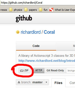
As mentioned in the previous step, we need to perform a 3x3 matrix inversion and multiplication. ActionScript's flash.geom.matrix class won't be able to help in this. Of course, we have a choice to utilise flash.geom.Matrix3D, class but I prefer the Coral library because I can pry into these custom classes and examine what's happening under the hood. I personally find this very useful whenever at doubt on proper use of commands even after reading the API documentation.

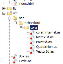
So download and place the unzipped Coral files into your project source folder.

Step 8: ActionScript Implementation

Here's a sample of the result. Try to reposition the red dots and see the quadratic curve redrawn to cross through all three points.

Step 9: Implementation Explained

You can find the full script in Draw_curve.as. The following ActionScript is just to enable mouse controls on the little dots.


public function Draw_Curve() 
{
    //setting up controls
    c1 = new Circle(0xFF0000); addChild(c1); c1.x = stage.stageWidth * 0.2; c1.y = stage.stageHeight >> 1;
    c2 = new Circle(0xFF0000); addChild(c2); c2.x = stage.stageWidth * 0.5; c2.y = stage.stageHeight >> 1;
    c3 = new Circle(0xFF0000); addChild(c3); c3.x = stage.stageWidth * 0.8; c3.y = stage.stageHeight >> 1;
    
    c1.addEventListener(MouseEvent.MOUSE_DOWN, move);
    c1.addEventListener(MouseEvent.MOUSE_UP, move);
    c2.addEventListener(MouseEvent.MOUSE_DOWN, move);
    c2.addEventListener(MouseEvent.MOUSE_UP, move);
    c3.addEventListener(MouseEvent.MOUSE_DOWN, move);
    c3.addEventListener(MouseEvent.MOUSE_UP, move);
    redraw()
}

private function move(e:MouseEvent):void {
    if (e.type == "mouseDown") {
        e.target.startDrag()
        e.target.addEventListener(MouseEvent.MOUSE_MOVE, update);
    }
    else if (e.type == "mouseUp") {
        e.target.stopDrag();
        e.target.removeEventListener(MouseEvent.MOUSE_MOVE, update);
    }
}

private function update(e:MouseEvent):void {
    redraw();
}

The core lies in the redraw function. I've highlighted the matrix operations and the quadratic function for the redraw process.

1
2	private function redraw():void
3	{
4	K = new Matrix3d( c1.x * c1.x, c1.x, 1, 0,
5	c2.x * c2.x, c2.x, 1, 0,
6	c3.x * c3.x, c3.x, 1, 0,
7	0, 0, 0, 1);
8	K.invert()
9	L = new Matrix3d( c1.y, 0, 0, 0,
10	c2.y, 0, 0, 0,
11	c3.y, 0, 0, 0,
12	0, 0, 0, 0);
13	L.append(K);
14
15	graphics.clear();
16	var points:Vector.<Number> = new Vector.<Number>;
17	var cmd:Vector.<int> = new Vector.<int>;
18	for (var i:int = 0; i < 200; i++) {
19	//current x
20	var x:Number = i * 2;
21
22	//f(x) = A (x^2) + B (x) + C
23	var y:Number = L.n11* x* x + L.n21 * x + L.n31 ;
24
25	points.push(x, y);
26	if (i == 0) cmd.push(1);
27	else cmd.push(2);
28	}
29	graphics.lineStyle(1);
30	graphics.drawPath(cmd, points);
31	}

So you can see that the matrix K was initialised and inverted before being appended onto matrix J.

The append() function multiplies the current matrix, J, with the input matrix, K, placed to its left. Another noteworthy detail is that we don't utilise all the rows and columns in K and J matrices. However since matrix inversion can only happen with a square matrix, we need to fill in the 4th row, 4th column element of K with 1. (There's no need to do this for J because we don't need its inversion in our calculation.) Thus, you can see all the other elements are 0 except for the first column.

Step 10: Graphing Cubic Curve

So that's all for drawing quadratic curves. Let's move on to cubic curves.

Again, we'll have a little revision of graphing these curves. Check out the following image:

Cubic graphed on Cartesian and Flash coordinate space.

When you compare this curve to that of quadratic, you will notice that it is steeper, and that a portion of the curve is below the x-axis. One half is mirrored vertically, compared to a quadratic.

Step 11: Cubic Coefficients

I've included the following Flash presentation to let you experiment with the coefficients of a cubic equation. Try tweaking the value of A from positive to negative and observe the difference in the curve produced.

Step 12: ActionScript Implementation

Here's the important section of the implementation of the graphing above:


private function redraw(A:Number, B:Number, C:Number, D:Number):void {
    for (var i:int = 0; i < 400; i++) {
        var x:Number = i - 200;
        points[i * 2] = x * 10 + stage.stageWidth >> 1;
        points[i * 2 + 1] = cubic1(x, A, B, C, D) + stage.stageHeight >> 1
        
        if (i == 0) drawCommand[i] = 1;
        else drawCommand[i] = 2;
    }
    graphics.clear();
    graphics.lineStyle(1);
    graphics.drawPath(drawCommand, points);
}

private function cubic1(x:Number, A:Number, B:Number, C:Number, D:Number):Number {
    //y = A(x^3) + B(x^2) + C(x) + D
    return A*x*x*x+ B*x*x + C*x +D
}

Again, it's difficult to position the cubic curve according to a set of points it crosses through. Once again, we refer to linear algebra for an alternative.

Step 13: Alternative Method

We know from Step 6 that the coefficients of a quadratic equation can be calculated based on three given points, and the curve drawn from it will cross through those points. A similar approach can be performed with any four given points to obtain a cubic equation:

\(S\ \left(S_x,\ S_y\right)\)
\(T\ \left(T_x,\ T_y\right)\)
\(U\ \left(U_x,\ U_y\right)\)
\(V\ \left(V_x,\ V_y\right)\)

Substitute these coordinates into (eq 2). Note that A, B, C, D are unknowns.

\[g(x) = Ax^3 + Bx^2 + Cx + D\ ... (eq\ 2)\]

\(S_y = A\left(S_x\right)^3 + B\left(S_x\right)^2 + C\left(S_x\right) + D\)
\(T_y = A\left(T_x\right)^3 + B\left(T_x\right)^2 + C\left(T_x\right) + D\)
\(U_y = A\left(U_x\right)^3 + B\left(U_x\right)^2 + C\left(U_x\right) + D\)
\(V_y = A\left(V_x\right)^3 + B\left(V_x\right)^2 + C\left(V_x\right) + D\)

But now we'll deal with a 4x4 matrix instead of 3x3 matrix:

\(
\begin{bmatrix}S_y \\T_y \\U_y \\V_y\end{bmatrix} =
\begin{bmatrix}
\left(S_x\right)^3 & \left(S_x\right)^2 & \left(S_x\right) & 1\\
\left(T_x\right)^3 & \left(T_x\right)^2 & \left(T_x\right) & 1\\
\left(U_x\right)^3 & \left(U_x\right)^2 & \left(U_x\right) & 1\\
\left(V_x\right)^3 & \left(V_x\right)^2 & \left(V_x\right) & 1\end{bmatrix}
\begin{bmatrix}A \\B \\C \\D\end{bmatrix} \\
P = QR \\
Q^{-1}P = Q^{-1}QR \\
Q^{-1}P = IR\\
Q^{-1}P = R
\)

Now we will utilise all elements in the 4x4 matrix for Q and the whole first column for P. Then Q is inversed and applied to P.

Step 14: ActionScript Implementation

Again, we set up the mouse controls to allow dragging of those points. When any of those points are being dragged, recalculation and redrawing of the curve constantly happen.


public function Draw_Curve2() 
{
    //setting up controls
    c1 = new Circle(0xFF0000); addChild(c1); c1.x = stage.stageWidth * 0.2; c1.y = stage.stageHeight >> 1;
    c2 = new Circle(0xFF0000); addChild(c2); c2.x = stage.stageWidth * 0.4; c2.y = stage.stageHeight >> 1;
    c3 = new Circle(0xFF0000); addChild(c3); c3.x = stage.stageWidth * 0.6; c3.y = stage.stageHeight >> 1;
    c4 = new Circle(0xFF0000); addChild(c4); c4.x = stage.stageWidth * 0.8; c4.y = stage.stageHeight >> 1;
    
    c1.addEventListener(MouseEvent.MOUSE_DOWN, move);
    c1.addEventListener(MouseEvent.MOUSE_UP, move);
    c2.addEventListener(MouseEvent.MOUSE_DOWN, move);
    c2.addEventListener(MouseEvent.MOUSE_UP, move);
    c3.addEventListener(MouseEvent.MOUSE_DOWN, move);
    c3.addEventListener(MouseEvent.MOUSE_UP, move);
    c4.addEventListener(MouseEvent.MOUSE_DOWN, move);
    c4.addEventListener(MouseEvent.MOUSE_UP, move);
    
    redraw();
}
private function move(e:MouseEvent):void {
    if (e.type == "mouseDown") {
        e.target.startDrag()
        e.target.addEventListener(MouseEvent.MOUSE_MOVE, update);
    }
    else if (e.type == "mouseUp") {
        e.target.stopDrag();
        e.target.removeEventListener(MouseEvent.MOUSE_MOVE, update);
    }
}

private function update(e:MouseEvent):void {
    redraw();
}

redraw is the crucial function where everything happened.

1
2	private function redraw():void
3	{
4	var left:Matrix3d = new Matrix3d(c1.x * c1.x* c1.x, c1.x* c1.x, c1.x , 1,
5	c2.x * c2.x * c2.x, c2.x* c2.x, c2.x , 1,
6	c3.x * c3.x * c3.x, c3.x* c3.x, c3.x , 1,
7	c4.x * c4.x * c4.x, c4.x* c4.x, c4.x , 1);
8	left.invert()
9	var right:Matrix3d = new Matrix3d(c1.y, 0, 0, 0,
10	c2.y, 0, 0, 0,
11	c3.y, 0, 0, 0,
12	c4.y, 0, 0, 0);
13	right.append(left);
14
15	//f(x) = A(x^3) + B (x^2) +C (x) + D
16	graphics.clear();
17	var points:Vector.<Number> = new Vector.<Number>;
18	var cmd:Vector.<int> = new Vector.<int>;
19	for (var i:int = 0; i < 200; i++) {
20	var x:Number = i * 2;
21	var y:Number = right.n11 * x * x * x+
22	right.n21 * x * x+
23	right.n31 * x +
24	right.n41;
25
26	points.push(x, y);
27	if (i == 0) cmd.push(1);
28	else cmd.push(2);
29	}
30	graphics.lineStyle(1);
31	graphics.drawPath(cmd, points);
32	}

Finally, let's look at the product. Click and move the red dots to see cubic curve drawn to pass through all those points.

Step 15: Polynomials of Higher Degree

We just gone through drawing polynomials of degree 2 and 3 (quadratic and cubic). From our experience, we can predict that calculation for polynomial of degree 4 (quintic) will require five points, which will require 5x5 matrix, and so on for polynomials of even higher degrees.

Unfortunately, Coral and flash.geom.Matrix3D only allow for 4x4 matrices, so you'll have write your own class if the need does come. It's seldom required in games, though.

Step 16: Dividing Regions

Let's try to apply our knowledge to divide regions on our stage. This requires some revision of equation inequalities. Check out the image below.

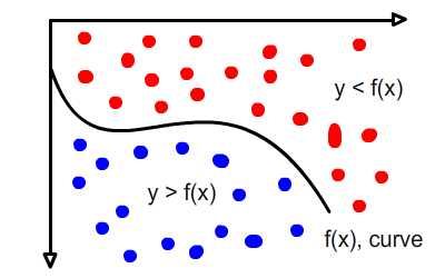
This image above shows a curve dividing the regions into two:

Blue region on top, where for each point y is greater than the equation of the curve.
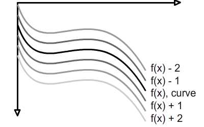
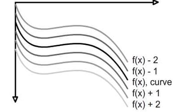
Red region at bottom, where for each point y is less than the equation of the curve.

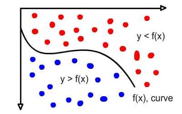
It's not hard to grasp this concept. In fact, you have already experimented on this in Step 11 as you tweaked the coefficients of the cubic formula. Imagine, in the coordinate system, that there is an infinite number of curves, all differentiated by just a slight change in D:

Step 17: ActionScript Implementation

So here's the sample of output for quadratic curve. You can try to move the red dot around and see the regions coloured.

Here's the important ActionScript snippet. Check out the full script in Region_Curve.as


private function redraw():void {
    var left:Matrix3d = new Matrix3d(c1.x * c1.x, 	c1.x, 	1, 	0,
                                     c2.x * c2.x, 	c2.x, 	1, 	0,
                                     c3.x * c3.x, 	c3.x, 	1, 	0,
                                     0, 			0, 		0, 	1);
    left.invert()
    var right:Matrix3d = new Matrix3d(c1.y, 	0, 	0, 	0,
                                      c2.y, 	0, 	0, 	0,
                                      c3.y, 	0, 	0, 	0,
                                      0, 	0, 	0, 	0);
    right.append(left);
    
    //D = A (x^2)+ B (x) +C 
    for each (var item: Circle in background) {
        var D:Number = right.n11* item.x * item.x + right.n21 * item.x + right.n31 ;
        //trace(background[i].y);
        if (item.y > D) item.color = 0;
        else item.color = 0xAAAAAA;
    }
}

Here's the sample with regard to cubic curve.

And the implementation that comes with it. Again, full script's in Region_Curve2.as


//D = A + B (x) +C (x^2)
for each (var item: Circle in background) {
    var D:Number = right.n11 * item.x * item.x * item.x;+ 
                                right.n21 * item.x * item.x +
                                right.n31 * item.x +
                                right.n41 
    //trace(background[i].y);
    if (item.y > D) item.color = 0;
    else item.color = 0xAAAAAA;
}

Step 18: Variations

How about some tweaks to change the color across different curves? Again, mouse click on the red dots and see the gradient changes across the screen.

Step 19: ActionScript Implementation

Here's the important ActionScript snippet extracted from Region_Curve3.as. First of all we'll want to find out the maximum and minimum offset from the original curve.


var max:Number = 0;
var min:Number = 0;
var Ds:Vector.<Number> = new Vector.<Number>;

//D = A(x^2) + B (x) +C 
for each (var item: Circle in background) {
    var D:Number = right.n11 * item.x * item.x + right.n21 * item.x + right.n31;
    var offset:Number = item.y - D;
    Ds.push(offset);
    
    if (item.y > D && offset > max) max = offset;
    else if (item.y < D && offset < min) min = offset;
}

Once done, we'll apply it to colouring the individual dots.


//color variations based on the offset
var color:Number
for (var i:int = 0; i < background.length; i++) {
    if (Ds[i] > 0) {
        color = Ds[i] / max * 255							//calculating color to slot in
        background[i].color = color<<16 | color<<8 | color;	//define a grayscale
    }
    else if (Ds[i] < 0)	{
        color = Ds[i] / min * 255;
        background[i].color = color<<16;	//define a gradient of red
    }
}

Conclusion

So that all for the drawing of curves. Next up, finding roots of a quadratic and cubic curve. Thanks for reading. Do share if you see some real life applications that takes advantage of this tutorial.