The Math and ActionScript of Curves: Roots

In the first tutorial of this series, we took a look at drawing curves using equations and AS3. Now, we're going to tackle solving those equations to find the roots of a curve - that is, the places where the curve crosses a given straight line. We can use this to predict collisions with curved surfaces, and to avoid "tunnelling" in Flash games.

Step 1: Quadratic Roots

First, time for some quick math revision. In this tutorial, we'll just accept and apply the methods we'll use, but interested readers can refer to Wikipedia's page on quadratic equations for information about the mathematical deriviations.

So \(f(x)\) is a quadratic function. If \(f(x)\) is equivalent to 0, \(x\) can be obtained by this formula:

\[Given\ f(x)\ = \ ax^2+bx+c,\ \]
\[f(x)\ =\ 0,\ x = \frac{-b \pm \sqrt{b^2 - 4ac}}{2a} \]

\(b^2 - 4ac\) is called the discriminant of the formula. If the discriminant is negative, the square root of the discriminant will produce imaginary roots, which we can't plot. Conversely, if the discriminat is positive, you will have real number roots and you'll be able to plot them onto the screen.

Step 2: Visualising Quadratic Roots

So what are roots? Well in our context they are nothing more than intersection points between the quadratic curve and a line. For example, suppose we are interested to find the intersection point(s) of the following set of equations:

\(
f(x)\ = \ ax^2+bx+c \\
g(x)\ = \ 0
\)

This is a typical scenario of looking for the intersection point(s) between a quadratic curve and the x-axis (because the x-axis is the line where y==0). Since by definition the intersection point(s) are shared by \(f(x)\) and \(g(x)\), we can conclude that \(f(x) = g(x)\) for the values of x that we are looking for.

It's then a trivial operation where you just substitute the functions and then apply the formula from Step 1 to obtain the roots. Now there are several possibilities we can anticipate as shown below.

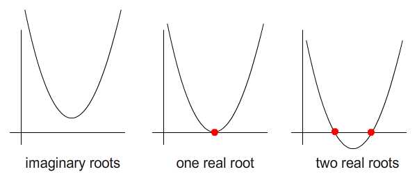
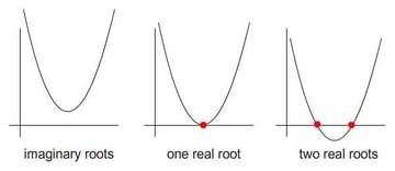
(As you can see, "imaginary roots" means, for our purposes, that the curve doesn't ever cross the x-axis.)

Now let's consider the case where \(g(x)\) is more than just a mundane horizontal line. Let's say it's a slanted line, \(g(x)\ =\ mx\ +\ d\). Now when we equate both functions, we'll need to do a little precalculation before the formula can be effectively applied.

\[
ax^2\ +\ bx + c\ =\ mx\ +\ d\\
ax^2\ +\ (\ b\ - m)\ x + (c\ -\ d)\ =\ 0
\]

I've included an interactive Flash presentation below so feel free to drag the red and blue dots. Yellow dots indicate the intersection points. You may need to position the curve and line to intersect each other in order for the yellow dots to appear.

Step 3: Plotting This With ActionScript

The full script can be found in Demo1.as; here I'll just explain a crucial extract of the code. Let's look at the AS3 for drawing the curve and line:


private function redraw():void 
{
    var cmd:Vector.<int> = new Vector.<int>;
    var coord:Vector.<Number> = new Vector.<Number>;
    
    //redraw curve;
    m1 = new Matrix3d(
        curve_points[0].x * curve_points[0].x, curve_points[0].x, 1, 0,
        curve_points[1].x * curve_points[1].x, curve_points[1].x, 1, 0,
        curve_points[2].x * curve_points[2].x, curve_points[2].x, 1, 0,
        0,0,0,1
    );
    
    m2 = new Matrix3d(
        curve_points[0].y, 0, 0, 0,
        curve_points[1].y, 0, 0, 0,
        curve_points[2].y, 0, 0, 0,
        0,0,0,1
    )
    
    m1.invert();
    m2.append(m1);
    quadratic_equation.define(m2.n11, m2.n21, m2.n31);
    
    for (var i:int = 0; i < stage.stageWidth; i+=2) 
    {
        if (i == 0) cmd.push(1);
        else		cmd.push(2);
        
        coord.push(i, quadratic_equation.fx_of(i));
    }
    
    //draw line
    n1 = new Matrix();
    n1.a = line_points[0].x; n1.c = 1;
    n1.b = line_points[1].x; n1.d = 1;
    
    n2 = new Matrix();
    n2.a = line_points[0].y; n2.c = 0;
    n2.b = line_points[1].y; n2.d = 0;
    
    n1.invert();
    n2.concat(n1);
    
    var x:Number = stage.stageWidth		//y = mx + c
    cmd.push(1);	coord.push(0, n2.a * 0 + n2.b);
    cmd.push(2);	coord.push(x, n2.a * x + n2.b);
    
    graphics.clear();
    graphics.lineStyle(1);
    graphics.drawPath(cmd, coord);
}

The bulk of ActionScript for drawing the curve from line 80~104 is largely borrowed from the previous tutorial, so I shall just explain a little about the code for drawing a line.

In the Flash presentation above, there are two interactive blue dots. Each of these has coordinates, and with both dots, a line is formed. Since both dots lie on the same line, they share a common slope and y-intercept to form one general line equation:

\[
y\ =\ mx\ +\ d,\\
m\ =\ slope,\ d\ =\ y-intercept
\]

We can use a little algebra to solve for the two unknowns, \(m\) and \(d\). Given the coordinates of the two blue dots as \((x_1,\ y_1)\) and \((x_2,\ y_2)\):

[latex]
y_1 = mx_1 + d\\
y_2 = mx_2 + d\\
[/latex]

[latex]
\begin{bmatrix}y_1 \\y_2\end{bmatrix} =
\begin{bmatrix}x_1 & 1\\x_2 & 1\end{bmatrix}
\begin{bmatrix}m \\d\end{bmatrix} \\
[/latex]

[latex]
\begin{bmatrix}x_1 & 1\\x_2 & 1\end{bmatrix}^{-1}
\begin{bmatrix}y_1 \\y_2\end{bmatrix} =
\begin{bmatrix}x_1 & 1\\x_2 & 1\end{bmatrix}^{-1}
\begin{bmatrix}x_1 & 1\\x_2 & 1\end{bmatrix}
\begin{bmatrix}m \\d\end{bmatrix} \\
[/latex]

[latex]
\begin{bmatrix}x_1 & 1\\x_2 & 1\end{bmatrix}^{-1}
\begin{bmatrix}y_1 \\y_2\end{bmatrix} =
I
\begin{bmatrix}m \\d\end{bmatrix}
[/latex]

(Note that a matrix with superscripted -1 refers to inverse of that matrix.)

So using this, \(m\) and \(d\) are calculated. We can can now draw the line by joining the coordinates \((0, y_3)\) and \((stage.stageWidth, y_4)\). How do you find \(y_3\) and \(y_4\)? Well now that \(m\), \(x\) and \(d\) are known, we can simply put all these values into the line general equation,

\(y\ =\ mx\ +\ d\)

..to get those \(y\)s.

Step 4: Calculate the Quadratic Roots

To calculate the position of the intersecting points, we shall use the formula from Step 1. This is done in EqQuadratic.as as the functions shown below:


/**Read-only
 * Discriminant of equation
 */
public function get discriminant():Number {
    //B*B-4*A*C
    return _B * _B - 4 * _A * _C;
}

/**
 * Performs calculation to obtain roots
 */
public function calcRoots():void {
    var disc:Number = this.discriminant
    
    //handle imaginary roots
    if (disc < 0) { 
        disc *= -1;
        var component_real:Number = -_B / (2 * _A);
        var component_imaginary:Number = Math.sqrt(disc) / (2 * _A);
        
        _root_i[0] = (component_real + "+ i" + component_imaginary).toString();
        _root_i[1] = (component_real + "- i" + component_imaginary).toString();
    }
    
    //handle real roots
    else {
        var sqrt:Number = Math.sqrt(disc);
        _root_R[0] = ( -_B + sqrt) / (2 * _A);
        _root_R[1] = ( -_B - sqrt) / (2 * _A);
    }
}

Further details of EqQuadratic.as:

Function	Type	Input Parameter	Functionality
EqQuadratic	Method	Nil	Class constructor
define	Method	Coefficients a, b and c of quadratic equation	Instantiate the coefficient values
fx_of	Method	Value of x	Returns \(f(x)\) of given \(x\) input.
calcRoots	Method	Nil	Performs calculation to obtain quadratic root
diff1	Method	\(x\) coordinate for the first degree differentiation	Differentiated \(f(x)\) of given \(x\) at the first degree.
diff2	Method	\(x\) coordinate for the second degree differentiation	Differentiated \(f(x)\) of given \(x\) at the second degree.
discriminat	Property, read only	Nil	Returns the value of discriminant, \(b^2 - 4ac\)
roots_R	Property, read only	Nil	Returns a Number vector for roots of real number. Elements are NaN if no real roots exist.
roots_i	Property, read only	Nil	Returns a String vector for roots of imaginary number. Elements are null if no imaginary roots exist.

Step 5: Plotting This With ActionScript

An example of utilising this EqQuadratic.as is in Demo1.as. After the initiation of EqQuadratic, we shall use it to calculate the roots. Then, after validating the presence of real roots, we'll use them to plot the yellow dots.

Now the roots refer to only the \(x\) component of the coordinates. To obtain the \(y\)s, guess what? Again, we put the values of \(m\), \(d\) (calculated earlier in Step 3) and \(x\) (from the roots) into the line general equation, \(y\ =\ mx\ +\ d\). Check out the corresponding code in line 135 and 136.


private function recalculate_reposition():void 
{
    quadratic_equation.define(m2.n11, m2.n21 - n2.a, m2.n31 - n2.b);
    quadratic_equation.calcRoots();
    
    var roots:Vector.<Number> = quadratic_equation.roots_R;
    
    if (!isNaN(roots[0]) && !isNaN(roots[1])) {
        intersec_points[0].x = roots[0]; intersec_points[0].y = n2.a * roots[0] + n2.b
        intersec_points[1].x = roots[1]; intersec_points[1].y = n2.a * roots[1] + n2.b
    }
    else {
        intersec_points[0].x = -100; intersec_points[0].y = -100;
        intersec_points[1].x = -100; intersec_points[1].y = -100;
    }
}

Step 6: Cubic Roots

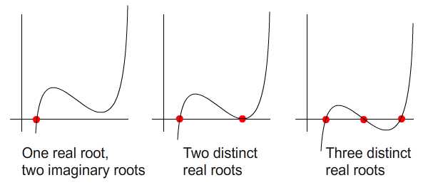
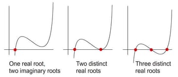
Cubic roots, not surprisingly, are the intersection points between a cubic curve and a line. But a cubic curve is a little different to a quadratic curve, and in this respect the possibilities for where intersections could be located are different.

The image below shows a cubic curve intersecting with the x-axis:

Possiblities of root locations on a cubic curve

Again, here's a little Flash presentation for you to experiment with. Red and blue dots can be dragged while the yellow ones just indicate the intersection points.

Step 7: General Formula for Cubic Roots

The general formula to find a cubic curve was discovered by Cardano. Although I'm enticed to elaborate on the details, I'll just point interested readers to the following links:

Wikipedia
Wolfram, and
Another userful PDF file.

Anyway, the EqCubic.as class implements this formula to resolve roots of cubic functions along with other mathematical utility functions. Generally all the attributes and methods for EqCubic.as follow the desciption as tabled in Step 4, because both classes EqQuadratic.as and EqCubic.as implement one common interface, IEquation.as, except for the details listed below.

Function	Difference
`define`	A total of four coefficients (a, b, c, d) to input for cubic equation; just three for quadratic equation.
`roots_R`, `root_i`	The total of real and imaginary roots is three for a cubic equation, but two for a quadratic equation.

Step 8: Plotting This With ActionScript

Here's the Actionscript implementation for the Flash presentation from Step 5. The full code is in Demo3.as.


private function redraw():void 
{
    var cmd:Vector.<int> = new Vector.<int>;
    var coord:Vector.<Number> = new Vector.<Number>;
    
    //redraw curve;
    m1 = new Matrix3d(
        curve_points[0].x * curve_points[0].x * curve_points[0].x, curve_points[0].x * curve_points[0].x, curve_points[0].x, 1,
        curve_points[1].x * curve_points[1].x * curve_points[1].x, curve_points[1].x * curve_points[1].x, curve_points[1].x, 1,
        curve_points[2].x * curve_points[2].x * curve_points[2].x, curve_points[2].x * curve_points[2].x, curve_points[2].x, 1,
        curve_points[3].x * curve_points[3].x * curve_points[3].x, curve_points[3].x * curve_points[3].x, curve_points[3].x, 1
    );
    
    m2 = new Matrix3d(
        curve_points[0].y, 0, 0, 0,
        curve_points[1].y, 0, 0, 0,
        curve_points[2].y, 0, 0, 0,
        curve_points[3].y, 0, 0, 0
    )
    
    m1.invert();
    m2.append(m1);
    cubic_equation.define(m2.n11, m2.n21, m2.n31, m2.n41);
    
    for (var i:int = 0; i < stage.stageWidth; i+=2) 
    {
        if (i == 0) cmd.push(1);
        else		cmd.push(2);
        
        coord.push(i, cubic_equation.fx_of(i));
    }
    
    //draw line
    n1 = new Matrix();
    n1.a = line_points[0].x; n1.c = 1;
    n1.b = line_points[1].x; n1.d = 1;
    
    n2 = new Matrix();
    n2.a = line_points[0].y; n2.c = 0;
    n2.b = line_points[1].y; n2.d = 0;
    
    n1.invert();
    n2.concat(n1);
    
    var x:Number = stage.stageWidth		//y = mx + c
    cmd.push(1);	coord.push(0, n2.a * 0 + n2.b);
    cmd.push(2);	coord.push(x, n2.a * x + n2.b);
    
    graphics.clear();
    graphics.lineStyle(1);
    graphics.drawPath(cmd, coord);
}

Again, the ActionScript commands to draw a cubic curve are exactly the same as explained in my previous article, whereas Actionscript commands to draw the line are already explained in Step 3 of this one.

Now let's move on to calculating and positioning the cubic roots:


private function recalculate_reposition():void 
{
    cubic_equation.define(m2.n11, m2.n21 , m2.n31 - n2.a, m2.n41 - n2.b);
    cubic_equation.calcRoots();
    
    var roots:Vector.<Number> = cubic_equation.roots_R;
    
    for (var i:int = 0; i < roots.length; i++) 
    {
        if (!isNaN(roots[i])) {
            intersec_points[i].x = roots[i]; intersec_points[i].y = n2.a * roots[i] + n2.b
        }
        else {
            intersec_points[i].x = -100; intersec_points[i].y = -100;
        }
    }
}

After instantiating cubic_equation in the constructor we proceed on to define its coefficients, calculate the roots, and store the roots in a variable.

One little note on the roots: there are a maximum of three real roots for a cubic equation, but not all real roots are present in all situation as some roots may be imaginary. So what happens when there's only one real root, for example? Well, one of the array of roots called from cubic_equation.roots_R will be a real number, while all the others will be Not a Number (NaN). Check out the highlighted ActionScript for this.

Step 9: Predicting Where an Object Will Collide With Curved Surface

A great application of calculating roots is projecting a collision point onto curved surface, as show below. Use the left and right arrow keys to steer the moving ship, and press up to accelerate. You will notice that collision points which would have happened in the past are slightly dimmed.

Step 10: Implementation

The idea is similar to that in my tutorial about predicting collision points. However, instead of colliding with a straight line, we're now using a curved line. Let's check out the code.

The snippet below is called every frame:


private function update(e:Event):void 
{
    //Steering left and right
    if (control == 1)  velo = velo.rotate(Math2.radianOf(-5));
    else if (control == 2)  velo = velo.rotate(Math2.radianOf(5));
    
    //manipulating velocity
    var currVelo:Number = velo.getMagnitude();
    if (increase == 0)  {
        currVelo -= 0.5; currVelo = Math.max(currVelo, 1); //lower bound for velocity
    }
    else if (increase == 1)  {
        currVelo += 0.5; currVelo = Math.min(currVelo, 5); //upper bound for velocity
    }
    velo.setMagnitude(currVelo);
    
    //update velocity
    ship.x += velo.x; ship.y += velo.y; ship.rotation = Math2.degreeOf(velo.getAngle());
    
    //reflect when ship is out of stage
    if (ship.x <0 || ship.x > stage.stageWidth) velo.x *= -1;
    if (ship.y <0 || ship.y > stage.stageHeight) velo.y *= -1;
    
    redraw();
    recalculate();
}

The core code lies in redraw and recalculate. Let's first see what's in redraw. It's the same one we had been using in previous demos. One little note on drawing the line. We saw in previous demos that two dots are needed to draw get the equation. Well, here we only have one ship. So to get the second point, just add the ship's velocity to its current position. I've highlighted the code for convenience.


private function redraw():void 
{
    var cmd:Vector.<int> = new Vector.<int>;
    var coord:Vector.<Number> = new Vector.<Number>;
    
    //redraw curve;
    m1 = new Matrix3d(
        w1.x * w1.x, w1.x, 1, 0,
        w2.x * w2.x, w2.x, 1, 0,
        w3.x * w3.x, w3.x, 1, 0,
        0,0,0,1
    );
    
    m2 = new Matrix3d(
        w1.y, 0, 0, 0,
        w2.y, 0, 0, 0,
        w3.y, 0, 0, 0,
        0,0,0,1
    )
    
    m1.invert();
    m2.append(m1);
    quadratic_equation.define(m2.n11, m2.n21, m2.n31);
    
    minX = Math.min(w1.x, w2.x, w3.x);
    maxX = Math.max(w1.x, w2.x, w3.x);
    
    for (var i:int = minX; i < maxX; i+=2) 
    {
        if (i == minX) cmd.push(1);
        else		cmd.push(2);
        
        coord.push(i, quadratic_equation.fx_of(i));
    }
    
    n1 = new Matrix();
    n1.a = ship.x; 			n1.c = 1;
    n1.b = ship.x + velo.x; n1.d = 1;
    
    n2 = new Matrix();
    n2.a = ship.y; 			n2.c = 0;
    n2.b = ship.y + velo.y; n2.d = 0;
    
    n1.invert();
    n2.concat(n1);
    
    var x:Number = stage.stageWidth		//y = mx + c
    cmd.push(1);	coord.push(0, n2.a * 0 + n2.b);
    cmd.push(2);	coord.push(x, n2.a * x + n2.b);
    
    graphics.clear();
    graphics.lineStyle(1);
    graphics.drawPath(cmd, coord);
}

Now for recalculate, I've done a little vector calculation to check whether the point is behind or in front of the ship. Check out the highlighted code:


private function recalculate():void 
{
    quadratic_equation.define(m2.n11, m2.n21 - n2.a, m2.n31 - n2.b);
    quadratic_equation.calcRoots();
    
    var roots:Vector.<Number> = quadratic_equation.roots_R;
    
    for (var i:int = 0; i < roots.length; i++) 
    {
        var reposition:Sprite = getChildByName("c" + i) as Sprite
        
        //conditions:
        //real root, value of x within the range
        if (!isNaN(roots[i]) && roots[i] > minX && roots[i] < maxX) {
            reposition.x = roots[i]; 
            reposition.y = n2.a * roots[i] + n2.b;
            
            //discriminating between future and already happened collision point
            var vec:Vector2D = new Vector2D(reposition.x - ship.x, reposition.y - ship.y);
            if (velo.dotProduct(vec) < 0) 	reposition.alpha = 0.4;
            else 							reposition.alpha = 1
        }
        else {
            reposition.x = -100; reposition.y = -100;
        }
    }
}

Step 11: Time-Based Collision Detection

Another great application is not quite as obvious as the first. To perform a more accurate collision detection, instead of basing our conclusion on the distance between two objects, we'll uae their time to impact. Why? Because "tunneling" can happen if we use distance based collision detection:

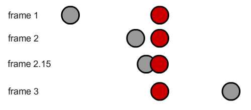
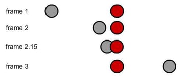
Consider a collision detection algorithm that's based on distance for two circles. Of the four frames shown, only frame 2.15 successfully detected collision between two circles. Why? Because the current distance between the gray and the red circles' centers is less than the sum of both circles' radii.

(Readers interested on more details on this topic can refer to this article.)

\[distance\ between\ circles\

The problem is caused by how Flash proceeds by one discrete frame at a time, which means that only frames 1, 2, and 3 will be successfully captured, and not the moments in between thos snapshots of time. Now the gray and red circles did not collide in these frames according to a distance-based calculation, so the red circle tunnels right through the gray one!

To fix this, we need a way to see the collision that occurred between frames 2 and 3. We need to calculate the time to impact between two circles. For example, once we check that time to impact is less than 1 frame at frame 2, this means that once Flash proceeds 1 frame forward collision or even tunneling will have definitely had taken place.

\[if\ time\ to\ impact,\ t,\ fulfills\ 0\

The question is, how do we calculate this time?

Step 12: Precalculations

I'll try to show my method as simply as possible.

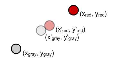
Given the scenario above, the two gray and red circles are currently located at \((x_{gray},\ y_{gray})\) and \((x_{red},\ y_{red})\). They are moving at \(v_{gray}\) and \(v_{red}\) respectively, and set on a collision path. We are interested to calculate the time taken, \(t\), for them to reach positions \((x'_{gray},\ y'_{gray})\) and \((x'_{red},\ y'_{red})\), indicated by the translucent gray and red circles, where the collision occurred.

\[
displacement_{future} = displacement_{present}+velocity*time\\
x'_{gray}=x_{gray}+v_{gray_x}*t\ ...(eq.\ 1)\\
y'_{gray}=y_{gray}+v_{gray_y}*t\ ...(eq.\ 2)\\
x'_{red}=x_{red}+v_{red_x}*t\ ...(eq.\ 3)\\
y'_{red}=y_{red}+v_{red_y}*t\ ...(eq.\ 4)
\]

Note that I've derived the horizontal and vertical components of \(v_{gray}\) into \(v_{gray_x}\) and \(v_{gray_y}\). Same goes with velocity of the red circle; check out this Quick Tip to get to know how these components are derived.

We still lack one relationship to bind all these equations together. Let's see the image below.

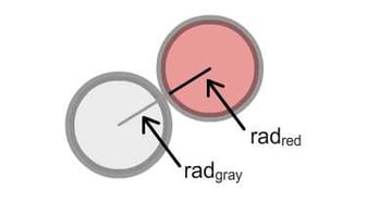
The other relationship goes back to Pythagoras. When both circles meet, the distance between both centers is exactly \(rad_{gray}\) plus \(rad_{red}\).

\[
Pythagoras'\ Theorem,\ z^2=x^2+y^2\\
(rad_{gray}+rad_{red})^2=(x'_{gray}-x'_{red})^2+(y'_{gray}-y'_{red})^2\ ...(eq.\ 5)\\
\]

This is where you substitute equations 1~4 into equation 5. I understand its quite daunting mathematically, so I've separated it out into Step 13. Feel free to skip it to arrive at the result at Step 14.

Step 13 (Optional): Mathematical Rigour

First, we establish the following identities.

\[
Identity,\\
(a+b)^2=a^2+2ab+b^2\ ...(id.\ 1)\\
(a-b)^2=a^2-2ab+b^2\ ...(id.\ 2)\\
\]

At all times, bear in mind that all mathematical symbols represent a constant except for time, \(t\), which is the subject of interest.

\(x_{gray},\ v_{gray_x},\ y_{red}, \) and so on are all defined in the scenario.

Next, we'll try to break our problem down term by term:

\[
(rad_{gray}+rad_{red})^2=(x'_{gray}-x'_{red})^2+(y'_{gray}-y'_{red})^2\\
Consider\ term\ (x'_{gray}-x'_{red})^2\ and\ utilising\ id.\ 2\\
(x'_{gray}-x'_{red})^2 = (x'_{gray})^2-2(x'_{gray})(x'_{red})+(x'_{red})^2\\
\]
\[
Consider\ term\ (x'_{gray})^2\\
(x'_{gray})^2\\
=(x_{gray}+v_{gray_x}*t)^2,\ utilise\ id.\ 1\\
=(x_{gray})^2+2(x_{gray})(v_{gray_x}*t)+(v_{gray_x}*t)^2
\]
\[
Consider\ term\ -2(x'_{gray})(x'_{red})\\
-2(x'_{gray})(x'_{red})\\
=-2(x_{gray}+v_{gray_x}*t)(x_{red}+v_{red_x}*t)\\
=-2[(x_{gray})(x_{red})+(x_{gray})(v_{red_x}*t)+(v_{gray_x}*t)(x_{red})+(v_{gray_x}*t)(v_{red_x}*t)]\\
=-2(x_{gray})(x_{red})-2(x_{gray})(v_{red_x}*t)-2(v_{gray_x}*t)(x_{red})-2(v_{gray_x}*t)(v_{red_x}*t)
\]
\[
Consider\ term\ (x'_{red})^2\\
(x'_{red})^2\\
=(x_{red}+v_{red_x}*t)^2,\ utilise\ id.\ 1\\
=(x_{red})^2+2(x_{red})(v_{red_x}*t)+(v_{red_x}*t)^2
\]

Now at a glance, we can easily see the highest power of \(t\) is 2. So we have ourselves a quadratic equation. Let's collect all the coefficients contributed by these three terms according to their powers.

\(t^2\)	\(t\)	\(t^0=1\)
\((v_{gray_x})^2\)	\(2(x_{gray})(v_{gray_x})\)	\((x_{gray})^2\)
\(-2(v_{gray_x})(v_{red_x})\)	\(-2(x_{gray})(v_{red_x})-2(v_{gray_x})(x_{red})\)	\(-2(x_{gray})(x_{red})\)
\((v_{red_x})^2\)	\(2(x_{red})(v_{red_x})\)	\((x_{red})^2\)

Let's analyse the coefficients with \(t^2\) and \(t^0\).

\[
(v_{gray_x})^2-2(v_{gray_x})(v_{red_x})+(v_{red_x})^2,\ recall\ id.\ 2\\
(v_{gray_x})^2-2(v_{gray_x})(v_{red_x})+(v_{red_x})^2 = (v_{gray_x}-v_{red_x})^2
\]
\[
(x_{gray})^2-2(x_{gray})(x_{red})+(x_{red})^2,\ recall\ id.\ 2\\
(x_{gray})^2-2(x_{gray})(x_{red})+(x_{red})^2 = (x_{gray}-x_{red})^2
\]

And that of \(t\).

\[
Simplify\\
a=(x_{gray}),\ b=(v_{gray_x})\\
c=(v_{red_x}),\ d=(x_{red})\\
2ab-2ac-2bd+2dc\\
=2[ab-ac-bd+dc]\\
=2[a(b-c)-d(b-c)]\\
=2[(b-c)(a-d)]\\
Resubstitute\\
2[(b-c)(a-d)] = 2(v_{gray_x}-v_{red_x})(x_{gray}-x_{red})
\]

Let's summarise in term of \((x'_{gray}-x'_{red})^2\)

\[
(x'_{gray}-x'_{red})^2\\
=(v_{gray_x}-v_{red_x})^2*t^2+2(v_{gray_x}-v_{red_x})(x_{gray}-x_{red})*t +(x_{gray}-x_{red})^2
\]

Note that this only caters for one term in \(eq.\ 5\). We'll need to perform the same process for another term \((y'_{gray}-y'_{red})^2\). Since they have the same algebraic form, the result should also be the same.
\[
(y'_{gray}-y'_{red})^2\\
=(v_{gray_y}-v_{red_y})^2*t^2+2(v_{gray_y}-v_{red_y})(y_{gray}-y_{red})*t +(y_{gray}-y_{red})^2
\]

Thus after rearrangement in terms of \(t\), \(eq.\ 5\) should be as follow.

\[
(rad_{gray}+rad_{red})^2=(x'_{gray}-x'_{red})^2+(y'_{gray}-y'_{red})^2\\
p=v_{gray_x}-v_{red_x}\\
q=x_{gray}-x_{red}\\
r=v_{gray_y}-v_{red_y}\\
s=y_{gray}-y_{red}\\
(p^2+r^2)*t^2+2(pq+rs)*t+(q^2+s^2-(rad_{gray}+rad_{red})^2) = 0
\]

Step 14: The Result

So from the previous step, through rigourous algebra we arrived at the following formula:

\[
p=v_{gray_x}-v_{red_x}\\
q=x_{gray}-x_{red}\\
r=v_{gray_y}-v_{red_y}\\
s=y_{gray}-y_{red}\\
(p^2+r^2)*t^2+2(pq+rs)*t+(q^2+s^2-(rad_{gray}+rad_{red})^2) = 0
\]

Now this is one huge quadratic formula. We'll try to group the coefficients into that accepted by EqQuadratic. Compare the two forms:

\[
ax^2+bx+c = 0\\
(p^2+r^2)*t^2+2(pq+rs)*t+(q^2+s^2-(rad_{gray}+rad_{red})^2) = 0\\
a = p^2+r^2)\\
b = 2(pq+rs)\\
c = (q^2+s^2-(rad_{gray}+rad_{red})^2)
\]

Step 15: Sample Implementation

So here's a Flash presentation to demonstrate the idea. You will see two particles on the stage, one gray and the other red. Both are connected to an arrow, indicating the magnitude and direction of velocity.

Click the "Next" button to progress one frame in time.
Click the "Back" button to revert one frame in time.

To alter the velocity of the particles, press:

"Up" and "down" to increase and decrease the velocity's magnitude, respectively.
"Left" and "right" to rotate the velocity.
"N" to switch which circle you control.

Finally, to toggle visibility of the arrows, press "V"

Step 16: A Note on the Quadratic Roots

There are two roots to the quadratic equation. In this context, we are interested in the real roots. However if the two particles are not set on collision path (both paths are parallel to each other), then imaginary roots will be produced instead of real roots. In this case, both real roots will remain NaN.

If both particles are set on a collision path, we will get two real roots. But what do these two roots represent?

Recall in Step 12 that we made used of Pythagoras's Theorem to tie \((x'_{gray},\ y'_{gray})\) and \((x'_{red},\ y'_{red})\) together into an equation. Well, there are two situations where the distance between two circles' centers are exactly the sum of both radii: one before collision and one after collision. Take a look at this image:

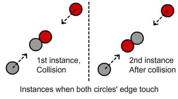
So which one do we choose? Obviously the first because we're not interested in the instance after collision. So we should always choose the lesser value of both roots and evaluate it. If the value is positive and less than 1, a collision will happen during the next frame. If the value is negative, the collision happened in the past.

Step 17: The ActionScript Explained

Let's look at the Actionscript implemented for this example. First, the variables.


//c1 is the gray circle
//c2 is the red circle
private var c1:Circle, c2:Circle;

//v1 is the gray circle's velocity
//v2 is the red circle's velocity
private var v1:Vector2D, v2:Vector2D, toggle:Boolean = true, usingV1:Boolean = true;

//tri1 will form the arrowhead of the v1
//tri2 will form the arrowhead of the v2
private var tri1:Triangle, tri2:Triangle;
private var container:Sprite;
private var eq:EqQuadratic;

Then the calculation of roots. You may want to cross check the following ActionScript with the variables above.

1
2	var p:Number = v1.x - v2.x;
3	var q:Number = c1.x - c2.x;
4	var r:Number = v1.y - v2.y;
5	var s:Number = c1.y - c2.y;
6
7	var a:Number = p * p + r * r;
8	var b:Number = 2 * (p * q + r * s);
9	var c:Number = q * q + s * s - (c1.radius + c2.radius) * (c1.radius + c2.radius);
10	eq.define(a, b, c);
11	eq.calcRoots();
12	var roots:Vector.<Number> = eq.roots_R;

Here's how you should interpret the roots:


//if no real roots are available, then they are on not on collision path
if (isNaN(roots[0]) && isNaN(roots[1])) {
    t.text = "Particles not on collision path."
}
else {
    var time:Number = Math.min(roots[0], roots[1])
    var int_time:int = time * 1000;
    time = int_time / 1000;
    
    t.text = "Frames to impact: "+time.toString() + "\n";
    if(time>1) t.appendText("Particles are closing...")
    else if (time > 0 && time < 1)  t.appendText("Particles WILL collide next frame!")
    else if (time < 0) t.appendText("Collision had already happened.");
}

Conclusion

So now we've studied quadratic and cubic roots in ActionScript, as well as taking a close look at two examples of how we can use the quadratic roots.

Thanks for taking the time to read this tutorial. Do leave a comment if you see other applications of quadratic roots (or any errors!)