The Math and ActionScript of Curves: Gradients and Normals

We've tackled drawing curves, and finding their quadratic and cubic roots, as well as handy applications for using quadratic roots within games. Now, as promised, we'll look at applications for finding cubic roots, as well as curves' gradients and normals, like making objects bounce off curved surfaces. Let's go!

Example

Let's take a look one practical use of this math:

In this demo, the "ship" bounces off the edges of the SWF and the curve. The yellow dot represents the closest point to the ship that lies on the curve. You can adjust the shape of the curve by dragging the red dots, and adjust the movement of the ship using the arrow keys.

Step 1: Shortest Distance to a Curve

Let's consider the scenario where a point is located near a quadratic curve. How do you calculate the shortest distance between the point and the curve?

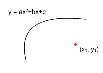
Well, let's start with Pythagoras's Theorem.

\[
Let\ the\ point\ be\ (x_p,\ y_p)\\
and\ call\ the\ closest\ point\ on\ the\ curve\ (x_c,\ y_c)\\
Then:\\
z^2 = x^2 + y^2\\
z^2 = (x_c-x_p)^2 + (y_c-y_p)^2\\
Given\ y_c=ax_c^2 + bx_c + c,\\
z^2 = (x_c-x_p)^2 + [(ax_c^2 + bx_c + c) -y_p]^2
\]

You can see that we have substituted \(y_c\) with the quadratic equation. At a glance, we can see the highest power is 4. Thus, we have a quartic equation. All we need to do is to find a minimum point in this equation to give us the shortest distance from a point to a quadratic curve.

But before that, we'll need to understand gradients on a curve...

Step 2: Gradient of a Curve

Before we look at the problem of minimizing a quartic equation, let's try to understand gradients of a curve. A straight line has only one gradient. But a quadratic curve's gradient depends on which point on the curve we refer to. Check out the Flash presentation below:

Drag the red dots around to change the quadratic curve. You can also play with the slider's handle to change the position of blue dot along x. As the blue dot changes, so will the gradient drawn.

Step 3: Gradient Through Calculus

This is where calculus will come in handy. You may have guessed that differentiating a quadratic equation would give you the gradient of the curve.

\[
f(x) = ax^2+bx+c\\
\frac{df(x)}{dx} = 2ax+b
\]

So \(\frac{df(x)}{dx}\) is the gradient of a quadratic curve, and it's dependant on the \(x\) coordinate. Well, good thing we've got a method to handle this: diff1(x:Number) will return the value after a single differentiation.

To draw the gradient, we'll need an equation to represent the line, \(y=mx+c\). The coordinate of the blue point \((x_p, y_p)\) will be substituted into the \(x\) and \(y\), and the gradient of the line found through differentiation will go into \(m\). Thus the y-intercept of line, \(c\) can be calculated through some algebra work.

Check out the AS3:


var x:Number = s.value
var y:Number = quadratic_equation.fx_of(s.value)
point.x = x;
point.y = y;

/**
 * y = mx + c;
 * c = y - mx;	<== use this to find c
 */
var m:Number = quadratic_equation.diff1(x);
var c:Number =  y - m * x;

graphics.clear();
graphics.lineStyle(1, 0xff0000);
graphics.moveTo(0, c);
graphics.lineTo(stage.stageWidth, m * stage.stageWidth + c);

Step 4: Coordinate Systems

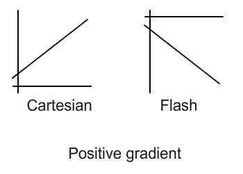
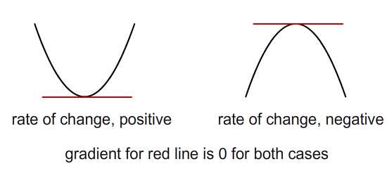
Always bear in mind of the inverted y-axis of Flash coordinate space as shown in the image below. At first glance, the diagram on right may seem like a negative gradient - but due to the inverted y-axis, it's actually a positive gradient.

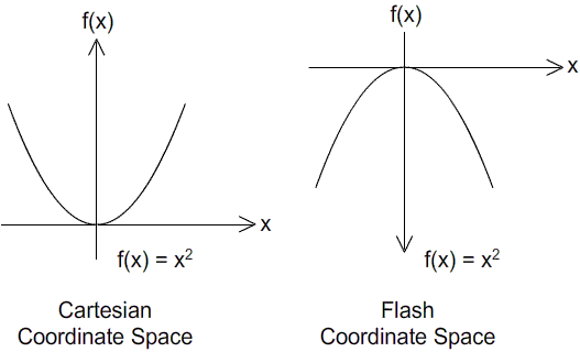
The same goes for the minimum point as indicated below. Because of the inverted y-axis, the minimum point in Cartesian coordinate space (at (0,0)) looks like a maximum in Flash coordinate space. But by referring to the location of origin in Flash coordinate space relative to the quadratic curve, it's actually a minimum point.

Step 5: Rate of Change for Gradient

Now let's say I'm interested in finding the lowest point on a curve - how do I proceed? Check out the image below (both figures are in the same coordinate space).

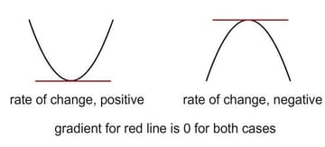
In order to get the minimum point, we'll just equate \(\frac{df(x)}{dx} = 0\), since by definition we're looking for the point where the gradient is zero. But as shown above, it turns out that the maximum point on a curve also satisfies this condition. So how do we discriminate between these two cases?

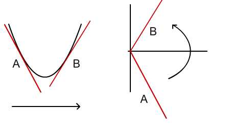
Let's try differentiation of the second degree. It'll give us the rate of change of the gradient.

\[
\frac{df(x)}{dx} = 2ax+b\\
\frac{df^2(x)}{dx^2} = 2a
\]

I'll explain with reference to the image below (drawn in Cartesian coordinate space). We can see that, as we increment along the x-axis, the gradient changes from negative to positive. So the rate of change should be a positive value.

We can also see that when \(\frac{df^2(x)}{dx^2}\) is positive, there's a minimum point on the curve. Conversely if the rate is negative, a maximum point is present.

Step 6: Back to the Problem

Now we are ready to solve the problem presented in Step 1. Recall the quartic equation (where the highest degree is 4) we arrived at:

\[
z^2 = (x_c-x_p)^2 + [(ax_c^2 + bx_c + c) -y_p]^2
\]

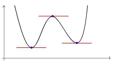
The same quartic equation, plotted

Remember, we are interested to find the minimum point on this curve, because the corresponding point on the original quadratic curve will be the point that's at the minimum distance from the red dot.

So, let's differentiate the quartic function to get to gradient of this curve, and then equate the gradient of this quartic function to zero. You will see that the gradient is actually a cubic function. I'll refer interested readers to Wolfram's page; for this tutorial, I'll just pluck the result of their algebra workings:

\[
\frac{d(z^2)}{dx}=
2(x_c-x_p) + 2(ax_c^2 + bx_c + c - y_p)(2ax_c+b)\\
\frac{d(z^2)}{dx}= 2a^2(x_c)^3+3ab(x_c)^2+(b^2+2ac-2ay_p+1)(x_c)+(bc-by_p-x_p)\\
Equate\ gradient\ to\ 0\\
\frac{d(z^2)}{dx}=0\\
2a^2(x_c)^3+3ab(x_c)^2+(b^2+2ac-2ay_p+1)(x_c)+(bc-by_p-x_p)=0\\
Compare\ with\ cubic\ equation\\
Ax^3+Bx^2+Cx+D=0\\
A = 2a^2\\
B=3ab\\
C=b^2+2ac-2ay_p+1\\
D=bc-by_p-x_p
\]

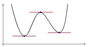
Solve for the roots of this (rather messy) cubic function and we'll arrive at the coordinates of the three blue points as indicated above.

Next, how do we filter our results for the minimum point? Recall from the previous step that a minimum point has a rate of change that's positive. To get this rate of change, differentiate the cubic function that represents gradient. If the rate of change for the given blue point is positive, it's one of the minimum points. To get the minimum point, the one that we're interested in, choose the point with the highest rate of change.

Step 7: Sample of Output

So here's a sample implementation of the idea explained above. You can drag the red dots around to customise your quadratic curve. The blue dot can also be dragged. As you move the blue dot, the yellow one will be repositioned so that the distance between the blue and yellow dots will be minimum among all points on the curve.

As you interact with the Flash presentation, there may be times where three yellow dots appear all at once. Two of these, faded out, refer to the roots obtained from the calculation but rejected because they are not the closest points on the curve to the blue dot.

Step 8: ActionScript Implementation

So here's the ActionScript implementation of the above. You can find the full script in Demo2.as.

First of all, we'll have to draw the quadratic curve. Note that the matrix m2 will be referred to for further calculation.


private function redraw_quadratic_curve():void 
{
    var cmd:Vector.<int> = new Vector.<int>;
    var coord:Vector.<Number> = new Vector.<Number>;
    
    //redraw curve;
    m1 = new Matrix3d(
        curve_points[0].x * curve_points[0].x, curve_points[0].x, 1, 0,
        curve_points[1].x * curve_points[1].x, curve_points[1].x, 1, 0,
        curve_points[2].x * curve_points[2].x, curve_points[2].x, 1, 0,
        0,0,0,1
    );
    
    m2 = new Matrix3d(
        curve_points[0].y, 0, 0, 0,
        curve_points[1].y, 0, 0, 0,
        curve_points[2].y, 0, 0, 0,
        0,0,0,1
    )
    
    m1.invert();
    m2.append(m1);
    quadratic_equation.define(m2.n11, m2.n21, m2.n31);
    
    for (var i:int = 0; i < stage.stageWidth; i+=2) 
    {
        if (i == 0) cmd.push(1);
        else		cmd.push(2);
        
        coord.push(i, quadratic_equation.fx_of(i));
    }
    
    graphics.clear();
    graphics.lineStyle(1);
    graphics.drawPath(cmd, coord);
}

And here's the one that implements the mathematical concept explained. c1 refers to a point randomly positioned on stage.


private function recalculate_distance():void 
{
    var a:Number = m2.n11;	
    var b:Number = m2.n21;
    var c:Number = m2.n31;
    
    /*f(x) = Ax^3 + Bx^2 +Cx + D
     */
    var A:Number = 2*a*a
    var B:Number = 3*b*a
    var C:Number = b*b + 2*c*a - 2*a*c1.y +1
    var D:Number = c * b - b * c1.y - c1.x
    
    quartic_gradient = new EqCubic();
    quartic_gradient.define(A, B, C, D);
    quartic_gradient.calcRoots();
    
    roots = quartic_gradient.roots_R;
    var chosen:Number = roots[0];
    
    if (!isNaN(roots[1]) && !isNaN(roots[2])) {
        
        //calculate gradient and rate of gradient of all real roots
        var quartic_rate:Vector.<Number> = new Vector.<Number>;
        
        for (var i:int = 0; i < roots.length; i++) 
        {
            if (!isNaN(roots[i])) 	quartic_rate.push(quartic_gradient.diff1(roots[i]));
            else 					roots.splice(i, 1);
        }
        
        //select the root that will produce the shortest distance
        for (var j:int = 1; j < roots.length; j++) 
        {
            //the rate that corresponds with the root must be the highest positive value
            //because that will correspond with the minimum point
            if (quartic_rate[j] > quartic_rate[j - 1]) {
                chosen = roots[j];
            }
        }
        
        //position the extra roots in demo
        position_extras();
    }
    else {
        
        //remove the extra roots in demo
        kill_extras();
    }
    intersec_points[0].x = chosen
    intersec_points[0].y = quadratic_equation.fx_of(chosen);
}

Step 9: Example: Collision Detection

Let's make use of this concept to detect the overlap between a circle and a curve.

The idea is simple: if the distance between the the blue dot and the yellow dot is less than blue dot's radius, we have a collision. Check out the demo below. The interactive items are the red dots (to control the curve) and the blue dot. If the blue dot is colliding with the curve, it will fade out a little.

Step 10: ActionScript Implementation

Well, the code is quite simple. Check out the full source in CollisionDetection.as.


graphics.moveTo(intersec_points[0].x, intersec_points[0].y);
graphics.lineTo(c1.x, c1.y);

var distance:Number= Math2.Pythagoras(
    intersec_points[0].x, 
    intersec_points[0].y, 
    c1.x, 
    c1.y)

if (distance < c1.radius)  c1.alpha = 0.5;
else                       c1.alpha = 1.0;

t.text = distance.toPrecision(3);

Step 11: Bouncing Off the Curve

So now that we know when collision will occur, let's try to program some collision response. How about bouncing off the surface? Check out the Flash presentation below.

You can see the ship (triangle shape), is surrounded by a circle (translucent blue). Once the circle collides with the curve, the ship will bounce off the surface.

Step 12: Controlling the Ship

Here's the ActionScript to control the ship.


public function CollisionDetection2() 
{
    /**
     * Instantiation of ship & its blue-ish circular area
     */
    ship = new Triangle();	addChild(ship);
    ship.x = Math.random() * stage.stageWidth;
    ship.y = stage.stageHeight * 0.8;
    
    c1 = new Circle(0x0000ff, 15);	addChild(c1);
    c1.alpha = 0.2;
    
    /**
     * Ship's velocity
     */
    velo = new Vector2D(0, -1);
    updateShip();
    
    stage.addEventListener(KeyboardEvent.KEY_DOWN, handleKey);
    stage.addEventListener(KeyboardEvent.KEY_UP, handleKey);
    stage.addEventListener(Event.EXIT_FRAME, handleEnterFrame);
    
    /**
     * The curve and the calculations
     */
    quadratic_equation = new EqQuadratic();
    
    curve_points = new Vector.<Circle>;
    populate(curve_points, 0xff0000, 3);
    
    intersec_points = new Vector.<Circle>;
    populate(intersec_points, 0xffff00, 3, false);
    
    redraw_quadratic_curve();
}

private function handleKey(e:KeyboardEvent):void 
{
    if (e.type == "keyDown") {
        if (e.keyCode == Keyboard.UP) isUp = true;
        else if (e.keyCode == Keyboard.DOWN) isDown = true;
        if (e.keyCode == Keyboard.LEFT) isLeft = true;
        else if (e.keyCode == Keyboard.RIGHT) isRight = true;
    }
    if (e.type == "keyUp") {
        if (e.keyCode == Keyboard.UP) isUp = false;
        else if (e.keyCode == Keyboard.DOWN) isDown = false;
        if (e.keyCode == Keyboard.LEFT) isLeft = false;
        else if (e.keyCode == Keyboard.RIGHT) isRight = false;
    }
}

private function handleEnterFrame(e:Event):void 
{
    /**
     * Control the magnitude
     */
    if (isUp) 		velo.setMagnitude(Math.min(velo.getMagnitude()+0.2, 3));
    else if(isDown)	velo.setMagnitude(Math.max(velo.getMagnitude()-0.2, 1));
    
    /**
     * Control the direction
     */
    if (isRight) velo.setAngle(velo.getAngle() + 0.03);
    else if (isLeft) velo.setAngle(velo.getAngle() - 0.03);
    
    recalculate_distance();
    
    if (distance < c1.radius) bounce();
    updateShip();
}

/**
 * Update ship's position, orientation and it's area (the blue-ish circle)
 */
private function updateShip():void {
    ship.x += velo.x;
    ship.y += velo.y;
    ship.rotation = Math2.degreeOf(velo.getAngle());
    
    c1.x = ship.x; 
    c1.y = ship.y;
    
    if (ship.x > stage.stageWidth || ship.x < 0) velo.x *= -1;
    if (ship.y > stage.stageHeight || ship.y < 0) velo.y *= -1;
}

You can see that the keyboard controls are updating flags to indicate whether the left, up, right, or down keys are being pressed. These flags will be captured by the enterframe event handler and update the magnitude and direction of the ship.

Step 13: Calculating the Reflection Vector

I've already covered the vector calculation of reflection vector in this post. Here, I shall just cover how to obtain the normal vector from gradient.

\[
\frac{df(x)}{dx}=gradient\\
line\ gradient=\frac{y}{x}\\
Assume\ gradient=0.5\\
y=0.5\\
x=1\\
Vector\ of\ left\ normal=
\begin{bmatrix}-1 \\0.5\end{bmatrix}\\
Vector\ of\ right\ normal=
\begin{bmatrix}1 \\-0.5\end{bmatrix}
\]

Step 14: ActionScript Implementation

So the ActionScript below will implement the mathematical concept explained in the previous step. Check out the highlighted lines:


private function bounce():void 
{
    var gradient:Number = quadratic_equation.diff1(intersec_points[0].x);
    var grad_vec:Vector2D = new Vector2D(1, gradient);
    
    var left_norm:Vector2D = grad_vec.getNormal(false);
    var right_norm:Vector2D = grad_vec.getNormal();
    var chosen_vec:Vector2D;
    
    if (velo.dotProduct(left_norm) > 0) chosen_vec = left_norm
    else 								chosen_vec = right_norm
        
    var chosen_unit:Vector2D = chosen_vec.normalise();
    var proj:Number = velo.dotProduct(chosen_unit);
    
    chosen_unit.scale(-2*proj);
    
    velo = velo.add(chosen_unit);
}

Conclusion

Well, thanks for your time! If you've found this useful, or have any questions, do leave some comments.